Parallelizing R with BatchJobs – An example using k-means

Gord Sissons, Feng Li

Many simulations in R are long running. Analysis of statistical algorithms can generate workloads that run for hours if not days tying up a single computer. Given the amount of time R programmers can spend waiting for results, getting acquainted parallelism makes sense.

In this first in a series of blogs, we describe an approach to achieving parallelism in R using BatchJobs, a framework that provides Map, Reduce and Filter variants to generate jobs on batch computing systems running across clustered computing environments.

Achieving parallelism with R on a single computer is straightforward. There are multiple approaches to multi-core or multi-socket parallelism including parallel, Rmpi, foreach and others. Where most of us run into difficulties is with distributed parallelism – running a model across many machines. While there are several approaches, not every data scientist is also a computer-scientist. Setting up distributed compute clusters can be time-consuming and difficult.

In this example we wanted to concentrate on a single application, but describe an approach that is applicable to a variety of use cases, and that can scale to arbitrarily large compute intensive problems and computing clusters in R.

Giving credit where credit is due

Before proceeding, we need to acknowledge the excellent work done by Glenn Lockwood – We’ve shamelessly borrowed his k-means coding example from http://glennklockwood.com/di/R-para.php as the basis of our example. To test parallelism, it is desirable to be able to scale the problem set, and Glenn’s k-means example fits the bill perfectly.

For readers already familiar with R and parallel techniques, what we will show here is similar to using foreach with doSNOW (the foreach adapter to a simple network of workstations clusters) but we argue in favor of using a BatchJobs with a workload manager for several reasons:

• It is at least as easy to setup as snow – easier I would argue
• There are multiple free, open-source workload managers – cost is not an issue
• The managed cluster can more easily scale to arbitrarily large workloads
• We can flex the cluster up and down at run-time (leveraging capabilities like Amazon spot pricing) by choosing the right open-source workload manager

Generating test data

K-means is a widely used algorithm used in many applications including machine-learning, biology and computer vision. The purpose of k-means clustering is to sift through observations, and iteratively group like-items together. It does this by partitioning observations, evaluating each clusters to find a new center, and re-evaluating and finding new clusters and centers until an optimal set of centers are found. It does this by using a least-squares method seeking to minimize the sum of the vector lengths for all data points associated with a cluster relative to its center.

There are plenty of real-world datasets that k-means can operate on, but for our purposes we wanted a simple example that we could easily scale up or down in size to experiment with different parallel computing approaches.

The R script below generates a text file called dataset.csv containing 250,000 rows of x, y pairs. The pairs are scattered in a normal distribution around five known center points. The script runs through 50,000 iterations, and for each iteration, a random data point is established around each of five pre-established centers yielding 250,000 separate data points.

The size of the dataset can be scaled by changing the nrow value in the script. Readers can experiment by changing the code below to use different centers, add additional clusters, or alter the size of the dataset. Running the script below in R studio generates our dataset.

#!/usr/bin/env Rscript
#
# gen-data.R - generate a "dataset.csv" for use with the k-means clustering
# examples included in this repository
#
nrow <- 50000
sd <- 0.5
real.centers <- list( x=c(-1.3, -0.7, 0.0, +0.7, +1.2),
y=c(-1.0, +1.0, 0.1, -1.3, +1.2) )
data <- matrix(nrow=0, ncol=2)
colnames(data) <- c("x", "y")
for (i in seq(1, 5)) {
x0 <- rnorm(nrow, mean=real.centers$x[[i]], sd=sd)
y0 <- rnorm(nrow, mean=real.centers$y[[i]], sd=sd)
data <- rbind( data, cbind(x0,y0) )
}

write.csv(data, file='dataset.csv', row.names=FALSE)

Running k-means against the dataset

Now that we have a dataset with 250,000 observations and known centers, we can use k-means to analyze it. The reason we call the script below serial.R is that by default R will not parallelize operations unless there are explicit provisions in the code to do so.

#!/usr/bin/env Rscript
#
# serial.R - Sample script that performs a kmeans analysis on the generated dataset.csv file
#
# ggplot2 is included so we can visualize the result
library(ggplot2)
 
#load the generated dataset
data <- read.csv('dataset.csv')
 
# run k-means and classify the data into clusters
start.time <- Sys.time()
result <- kmeans(data, centers=5, nstart=100)
end.time <- Sys.time()
 
time.taken <- end.time - start.time
print(time.taken)
 
# print the cluster centers based on the k-means run
print(result$centers)
 
# present the data as a visual plot
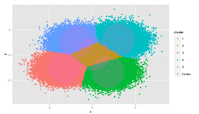
data$cluster = factor(result$cluster)
centers = as.data.frame(result$centers)
plot = ggplot(data=data, aes(x=x, y=y, color=cluster )) + geom_point() + geom_point(data=centers, aes(x=x,y=y, color='Center')) + geom_point(data=centers, aes(x=x,y=y, color='Center'), size=52, alpha=.3, show_guide=FALSE)
print(plot)
 

The serial.R script reads the dataset, and runs k-means looking for an arbitrary number of centers. We know the nature of the dataset in this case, but with unknown data, analysts might run k-means repeatedly looking for the optimal numbers of centers.

A key parameter in the k-means calculation is nstart. K-means works by choosing random centers as starting points, however the choice of centers can affect the result. To find the optimal result the algorithm needs to be run repeatedly with multiple randomly generated sets of centers. In the example above we are essentially running k-means 100 times (by setting nstart=100) and finding the best result that minimizes the distance between individual data points and the resulting centers of clusters.

We measure the time taken to exectute k-means, and take the extra step of using the ggplot2 package to visualize the results.

We run this script above, by sourcing it in R-studio as shown.

> source ('Rexamples/serial.R')
Time difference of 3.681569 mins
x           y
1 -1.31702692 -1.01035368
2 0.03388885 0.05849527
3 0.72134220 -1.33543312
4 1.21512570 1.21465315
5 -0.74567205 1.05607375
 
>

After 223 seconds of execution time, the five computed centers are obtained and data results are plotted as shown below. Clearly the model has worked as expected returning the centers from our known dataset and re-grouping the data points about their centers. The model is not perfect, but returns centers close to the values expected.

If we run the Linux command “top” on the host running the R studio server during execution, we see one of the challenges with R. Only one processor core is involved while other cores sit idle.

top - 14:37:08 up 11 days, 56 min, 4 users,   load average: 0.99, 0.56, 0.24
Tasks: 225 total,   2 running, 223 sleeping,   0 stopped,   0 zombie
Cpu0 :100.0%us,   0.0%sy, 0.0%ni, 0.0%id,   0.0%wa, 0.0%hi, 0.0%si,   0.0%st
Cpu1 : 0.0%us,   0.3%sy, 0.0%ni, 99.0%id, 0.7%wa,   0.0%hi, 0.0%si, 0.0%st
Cpu2 : 0.0%us,   0.0%sy, 0.0%ni,100.0%id, 0.0%wa,   0.0%hi, 0.0%si, 0.0%st
Cpu3 : 0.3%us,   0.3%sy, 0.0%ni, 99.3%id, 0.0%wa,   0.0%hi, 0.0%si, 0.0%st
Mem:   3857760k total, 1661896k used, 2195864k free,   186492k buffers
Swap: 3997692k total,     5612k used, 3992080k free,   676448k cached<

Ideally we’d like to use all of our processor cores, and multiple cores across multiple machines to complete the calculation as quickly as possible.

Parallelizing the calculation

The previous example was simple. It had known centers, a known number of clusters, and the data involved had only two dimensions. We can imagine the need to run larger and more complex multi-dimensional problems, and to run them not once, but multiple times.

To provide a multi-node example, we add a second computer with four cores and join it with the first machine to build a two node cluster with eight cores. The small two node cluster could be built with snow, but in this example we elected to use OpenLava, a free workload manager that is easy to setup and configure.

We’ve skipped the details of the setup here in the interest of keeping things brief, but we essentially performed the following steps.

• Download OpenLava from http://www.teraproc.com. You can also get OpenLava from org and compile it yourself if you choose
• Followed the installation directions provided with the free Teraproc .rpm file
• NFS exported the /home directory from the first host and mounted it on a second so that both nodes on the cluster shared a common file system

If you want to setup your own cluster locally or on Amazon, you can read a blog explaining the process here to manually setup a cluster. Another blog here explains how to setup an OpenLava cluster entirely for free using Amazon’s free tier. An even easier approach (that can also be free my using AWS free-tier machine types) is to provision a cluster using the Teraproc R cluster-as-a-service offering and plugging details of your amazon web services account into the setup screen at teraproc.com. Teraproc deploys a ready to run R cluster complete with OpenLava, OpenMPI, NFS, R-Studio server, Shiny and all the parallel R packages pre-configured.

In our two node test cluster, the R Studio server runs on our cluster node called “master”. The node called master is also acting as the OpenLava master and is linked to a second compute host called compute1.

The script batch-kmeans.R below has been adapted to run using the R package BatchJobs. BatchJobs is available on CRAN and can be easily installed in R Studio using install.packages(‘BatchJobs’) command.

You will need to configure a start-up script called .BatchJobs.R in your home directory with specifics about your workload manager. OpenLava is explicitly supported by BatchJobs along with other schedulers including UNIVA GridEngine, Platform LSF, PBS Pro and others. The contents of these files are omitted for brevity, but you can download a zip file with the source code and configuration files if you want to replicate this test on your own cluster.

 

#!/usr/bin/env Rscript
#
library("BatchJobs")
library(parallel)
library(ggplot2)
# read the dataset generated by gen-data.R - this is not really necessary for execution
# of the jobs, but we want to have the datasets available in the current R instance to plot
data <- read.csv('/home/gord/dataset.csv')
 
# this is the function that represents one job
parallel.function <- function(i) {
set.seed(i)
data <- read.csv('/home/gord/dataset.csv')
result <- kmeans( data, centers=5, nstart=10 )
result
}
 
# Make registry for batch job
reg <- makeRegistry(id="TPcalc")
ids <- batchMap(reg, fun=parallel.function, 1:10)
print(ids)
print(reg)
 
# submit the job to the OpenLava cluster
start.time <- Sys.time()
done <- submitJobs(reg)
waitForJobs(reg)
 
# Load results of all "done" jobs
done <- findDone(reg)
results <- reduceResultsList(reg, use.names='none')
temp.vector <- sapply( results, function(results) { results$tot.withinss } )
final_result <- results[[which.min(temp.vector)]]
end.time <- Sys.time()
time.taken <- end.time - start.time
print(time.taken)
 
# show the results
print(final_result$centers)
# plot the results
data$cluster = factor(final_result$cluster)
centers = as.data.frame(final_result$centers)
plot = ggplot(data=data, aes(x=x, y=y, color=cluster )) + geom_point() + geom_point(data=centers, aes(x=x,y=y, color='Center')) + geom_point(data=centers, aes(x=x,y=y, color='Center'), size=52, alpha=.3, show_guide=FALSE)
print(plot)
# clean up after the batch job by removing the registry
removeRegistry(reg,"no")

The following changes are required to adapt the serial.R script for parallel execution with BatchJobs.

• We include the library BatchJobs
• We move the k-means calculation into a function that can be parallelized being careful load the dataset inside the function since threads will execute on different machines and need their own copy of the data (each node has access to the shared file system where dataset.csv is located via NFS)
• Note that rather than calling kmeans once with 100 different random centers, we are calling kmeans ten times with 10 different random centers, essentially parallelizing the same calculation
• As housekeeping for our batch environment, a few lines are required to create a registry that will hold information about the executing batch job. This registry is created on the shared /home file system available to each cluster host. We use “batchMap()” to setup ten separate jobs that will call our function containing the kmeans simulation. Each kmeans call will have nstart value set to ten so that we are still computing kmeans with 100 random starts in total.
• We then submit the jobs and use the convenient BatchJobs function “waitforJobs()” that blocks until all jobs on the cluster are complete.
• Once the jobs are done, we combine the results into a single list for post-processing and find the results that are more optimal based on the lowest total vector lengths.

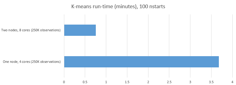
The output executing the parallel version of the script is shown below. Rather than taking over three minutes as was the case in our serial example, running the same problem as ten parallel chunks on the OpenLava cluster takes approximately 45 seconds – a dramatic improvement.

 

> source ('Rexamples/batch_kmeans.R')
Creating dir: /home/gord/TPcalc-files
Saving registry: /home/gord/TPcalc-files/registry.RData
Adding 10 jobs to DB.
[1] 1 2 3 4 5 6 7 8 9 10
Job registry: TPcalc
Number of jobs: 10
Files dir: /home/gord/TPcalc-files
Work dir: /home/gord
Multiple result files: FALSE
Seed: 284429578
Required packages: BatchJobs
Saving conf: /home/gord/TPcalc-files/conf.RData
Submitting 10 chunks / 10 jobs.
Cluster functions: LSF.
Auto-mailer settings: start=none, done=none, error=none.
Writing 10 R scripts...
SubmitJobs |++++++++++++++++++++++++++++++++++++++++++++++++++++++++++++++++++++++++++++++++++++++| 100% (00:00:00)
Sending 10 submit messages...
Might take some time, do not interrupt this!
Waiting [S:0 D:10 E:0 R:0] |+++++++++++++++++++++++++++++++++++++++++++++++++++++++++++++++++++++++| 100% (00:00:00)
 
Reducing 10 results...
reduceResults |+++++++++++++++++++++++++++++++++++++++++++++++++++++++++++++++++++++++++++++++++++| 100% (00:00:00)
 
Time difference of 0.758468 mins
x           y
1 0.03388885 0.05849527
2 -0.74567205 1.05607375
3 0.72134220 -1.33543312
4 1.21512570 1.21465315
5 -1.31702692 -1.01035368
 
>

From the perspective of the user in R-studio, their experience was essentially the same. They still ran the job interactively (even though execution behind the scenes was done in batch) and they received the same result. For longer running jobs, execution can be asynchronous using commands like showStatus() to monitor progress while continuing to be productive doing other work in R studio.

Monitoring usage on the master host and compute1 hosts during execution showed that both nodes were near 100% busy when jobs were running. This time the CPU utilization shows up in the NICE column (NI) in the top utility. This is another benefit of running under the OpenLava workload manager – the simulations are running at a lower priority so that our host computers are still able to respond to commands while the compute intensive jobs are executing.

top - 16:13:45 up 11 days,   2:33, 3 users, load average: 1.50, 0.52, 0.37
Tasks: 241 total,   5 running, 235 sleeping,   0 stopped,   1 zombie
Cpu0 : 0.3%us,   2.0%sy, 97.7%ni, 0.0%id, 0.0%wa,   0.0%hi, 0.0%si, 0.0%st
Cpu1 : 0.3%us,   4.3%sy, 95.3%ni, 0.0%id, 0.0%wa,   0.0%hi, 0.0%si, 0.0%st
Cpu2 : 0.0%us,   3.0%sy, 97.0%ni, 0.0%id, 0.0%wa,   0.0%hi, 0.0%si, 0.0%st
Cpu3 : 0.0%us,   2.6%sy, 97.4%ni, 0.0%id, 0.0%wa,   0.0%hi, 0.0%si, 0.0%st
Mem:   3857760k total, 2456880k used, 1400880k free,   191396k buffers
Swap: 3997692k total,     5612k used, 3992080k free,   827300k cached

 

Running OpenLava commands during the execution of the job shows the state of the cluster. The small two node cluster is completely busy with four parallel components running on each of the two nodes exploiting all four cores to maximize parallelism.

[root@master ~]# bhosts
HOST_NAME           STATUS       JL/U   MAX   NJOBS   RUN SSUSP   USUSP   RSV
compute1             closed         -     4       4     4     0       0     0
master               closed         -     4       4     4     0       0     0
[root@master ~]#

 

Tallying the results

Adding a second cluster node and using BatchJobs() with an open source workload manager delivers impressive results.

Our 10-way parallel model resulted in reducing the run-time from approximately 223 seconds to 46 seconds as shown below. This represents only about 20% of the run-time or a 5-fold reduction in the compute time. Presumably with ten cores our model would have completed in even less time.

In future posts I’ll show how we can accelerate more complex R machine learning algorithms like randomForest and how we can leverage MPI in R to run algorithms in parallel across multiple hosts as a single job, while sharing cluster resources with other simulations